Snuffler: Destripe Filtering

In my last post, I said that I would try and talk about Snuffler a bit more, so here is a post about a certain type of filtering in Snuffler, called 'Destripe'. This filter is used for processing magnetometry data. The most common type of magnetometry sensor is the fluxgate sensor, which is constructed of a metal ring with wire wound around it. The sensor is cheap to make and sensitive, but the downside is, it is directional, i.e. the reading will change according to the direction it is facing, effectively drowning out the slight changes you are trying to observe with what is effectively just a fluxgate compass.

The way to get around this problem is to use a gradiometer setup, where two sensors are arranged one above the other, and aligned so that when the device is turned, the earths magnetic field will affect both sensors equally, so that when you take the reading of one sensor away from the other, you will be left with the minor variations in reading from the sensor closest to the ground, which is just what you want.

Of course, in order for the gradiometer setup to function correctly, the two sensors must be perfectly aligned, and there are two ways of going about this, both of which use something called a zero point. A zero point is a magnetically sterile point on the ground where the device can be faced towards the cardinal compass points in order to balance it correctly. Such a point can be found by scanning around for one.

The first balancing method, used by devices such as the Geoscan FM256, uses physical balancing. The physical alignment of the sensors is adjustable, and these are manually adjusted according to the readings visible to the user of the device, which is quite fiddly.

The second balancing method, used by devices such as the Bartington GRAD601, uses electronic balancing. The fluxgate sensors are physically fixed within the sensor columns, rather than physically adjustable as above. The machine will get the user to point the device in various directions and record the readings. It can then compensate by adjusting any readings you get according to any deficiencies in the balancing process.

The place you may have chosen for your zero point may not be magnetically sterile, so it is worth making sure that in all directions, the readings you get at that point are broadly the same. If your zero point is not good enough, scan around for another one.  I personally try and get the readings all under 1nT, but that is a matter for personal preference. Filtering will take care of the rest. Of course there are some people why don't like filtering spoiling the purity of their lovely data. Personally I think these people are up themselves, but that is just me. You are unlikely to get close enough to 0nT in all directions when you balance your machine, and this will lead to a stripeyness on your results, which is where the destripe filter comes in. Like with most filtering, artifacts can be produced as a result, which is why the up-themselves brigade don't like them, but as long as you understand what the filters do, and what they have done to your data, there will be no problem with interpretation.

In its most basic form, destriping will average the readings in each line, and then adjust that line so that the average will be zero. On destripe options window in Snuffler, this is the 'Zero Mean Line' option. For the average survey, this is probably ok, but there is a better way. Each sensor column facing in each direction will have its own bias, so if you are zig-zagging (walking in two directions) with a GRAD601-2 (two sensor columns), you will have a total of four separate biases, which is a bias per sensor/direction. The other two destripe modes in Snuffler take account of this. The 'Grid Per Sensor/Direction' mode will average the sensor/direction biases across a grid, whilst the 'Image Per Sensor/Direction' mode will take the average across the entire image. For the sensor/direction averages to work, Snuffler has to know about the sensors and progression across the grid. For each image, it will get this when your view is created from the import data. On old versions of the software, this transfer of information did not happen, so if the sensor/direction options are not available to you, try recreating the Grids, Map and View from the original import data.

So why is averaging per sensor/direction approach to destriping better than averaging each line? I will give you two examples why. Take the below image, which is raw data showing some nasty metal water pipes.

Ewww, nasty pipes. Anyway, the problem with this data is that the large areas of positive or negative readings will produce a bias in the averaging, causing artifacts to appear when the 'Zero Mean Line' option is used, as you can see below.

Snuffler tries to reduce this by clipping the data used for averaging to the display limits, which in the latest version of the software is automatically set to +/-2nT for magnetometry data. This will only help so much however, leaving the light and dark areas shown above. If these local variations to the average are spread out using the sensor/direction averaging, you will get the below instead. This is sensor/direction per grid.

Well that's not much better, I hear you cry. You will see however, that the individual grids (there are four here) are mostly stripe free, even though they don't quite agree with eachother. So lets try sensor/direction per image.

It's not perfect, and is slightly stripier than the previous image, but at least the grids match eachother. The downside of averaging across the image is that instruments will drift, so in most cases, averaging per grid will be better, but where there is extreme disruption, as in the data set above, averaging per image may help. In most cases, averaging per grid will give you the best result, and from the latest of Snuffler, this will be the default mode selected.

So that is an example of how the sensor/direction model helps with features that you don't want. Now here is an example of how it can help with features that you do want. Take this set of raw data. You can see, despite the striping, that there is a broad enclosure ditch.

The trouble is, when a linear feature you are surveying is aligned to the way you are walking, the 'Zero Mean Line' method can wipe it out, as you can see below.

That's not much help is it, but if we take averages acros the grid per sensor/direction rather than per line, we get the following.

That's a lot better isn't it. You can still see the feature and the data is destriped.

As I said at the start of this blog post, it helps if you understand what the filters are doing when you use them, you will get much better results out of it. It is easy for me, because I wrote it, so I understand perfectly. I hope this article goes some way to helping all you Snuffler users out there understand how it works.

Version 1.0 of Snuffler Released

The title of this blog is Archaeological Geophysics with Snuffler, and yet I have hardly mentioned Snuffler at all. For those of you who don't know the history of it, I'll talk a bit about that now.

I got into archaeology the way a lot of people do, by joining a local amateur society and digging holes in the ground. I started out digging with the Mid-Sussex Field Archaeology Team and Brighton and Hove Archaeological Society. These societies had been doing a bit of geophysics, and due to my technical background, I soon became interested in this side of things. Disliking the commercial software option available at the time, I decided to start writing my own in my spare time. I called it Snuffler, because geophysics is like a wild boar snuffling for truffles. That was back in 2001. Over a decade later, a lot of new features have been added, and the software has grown from simply a personal project to something used by amateur archaeologists around the world. I decided to make it free for three reasons. Firstly, it was a personal project for me, rather than a commercial enterprise, so if anyone else got something out of it, then that was great. Secondly, as it became more than just a personal project, I thought it was worthwhile helping all the people with limited resources, who couldn't afford the commercial software options. Thirdly, I really couldn't be bothered messing about with the copy protection needed to make it commercially viable.

All of this leads me to the point of this post. The latest version of the software, version 1.0, has now been released. Yes, it's finally out of beta after all these years. I'm sure there are still bugs in there though, but hopefully not too many. So what's new in this version?

Firstly, there is now download support for the Geoscan FM256. Since I don't have one of these myself (I use a Bartington), I haven't personally tested it, so if you have problems, do let me know.

Secondly, PNG file export has been updated. As well as being able to set the invalid colour to transparent, you can now export a GIS World File, so that your PNG image can be loaded into GIS software.

As usual, you can download the software at http://www.sussexarch.org.uk/geophys/snuffler.html.

Over the next few months, I will hopefully be remedying the lack of talk about Snuffler itself with a few posts about things like filtering.

Latest Results: Ringmer

I've recently connected with the Roman Ringmer Study Group, as their area of expertise is where I am looking for a Roman road. To start them off however, I helped them out with something they are currently working on, which was possible a field with something Roman in it, but also has something medieval. According to records, there is a medieval manor house, which was taxed for no less that 8 hearths, which is quite a lot of hearths, and here are the results.

All of you who know me know that something that modern isn't really my bag, so I'm strugglinga bit to interpret this a bit. There are linear features, which seem to be composed of dipole noise rather than the usual ditches, so these could be wall lines composed of a magnetic material such as brick. The strongest rectangular feature is 20 metres wide and 40 metres extending into the field, with possible subdivisions inside. There is another weaker feature stretching a further 30 metres at the same width, possible containing a 9mx19m outbuilding in the SE corner. There is noise suggesting more activity either side of the main features, but none of it is clear. Does anyone out there know more about medieval than me? If so, what are your thoughts?

Latest Results: Rocky Clump

For those of you who haven't heard of Rocky Clump (i.e. not Sussex archaeologists), it's a Roman farming settlement near the city of Brighton that has been under excavation by the Brighton and Hove Archaeological Society for the past billion years (or so it seems). Not quite as rich as a villa, but interesting nevertheless. The site is famous for a vast array of ditches that seem to make no sense, and some sarsen stones in a clump of trees after which the site is named. After several years digging up ditches to the north of the clump, BHAS started digging to the south in 2011. Many, many years ago, I did a large resistivity survey in the south field which showed up a large number of features, which you can see the results of below. Click the image for a larger version.

Whilst there is a lot going on in the image, a lot of it is geological. Readers of this blog may remember a post I wrote about an annoying form of geology known as clay-with-flints. This nasty stuff will make you think you have features everywhere, until you dig them up. There is an upside though. Normally magnetometry will not work on chalk, as there are no magnetic particles in the soil to form a contrasting reading when a ditch cuts the geology. The presence of the clay-with-flints introduces those magnetic particles, allowing magnetometry to work. I resurveyed part of the field today, to see if I could work out which of the features were geology and which were archaeology. You can see the results below.

Just look at all those lovely ditches. There is a small settlement enclosure in the middle, possibly within the corner of a field boundary. The ditch to the north that was visible on the resistivity is also visible on the magnetometry, but the large low resistance area that it passed through is now looking like geology, but I can't be sure about that. Further to the west are three ditches, one of which takes a curve to the south, and a possible east-west trackway formed by two further ditches. Of the two large low resistance features near the clump, the north-west one has transformed itself into a series of small ditch features and is most likely archaeological. The south-east one is a bit of a mess and is most likely geological, but again I can't be sure. There are plenty of dark blobs that represent the clay-with-flints, which stand in stark contrast to the fainter archaeology. One particular faint feature to take note of is just to the north-west of the settlement enclosure. It is about 6m x 4.5m, and could well be part of the settlement. BHAS have stripped the topsoil for a new excavation this year, which shows up well as a giant white reverse L shaped feature.

Walking Around Your Geophysics Results II

Hello everybody,

Do you remember me writing this long and complicated blog post about how to walk around your geophysics results using a mobile device? Well you can forget about all that. I recently saw this blog post from Google, which suggested that you can now open kml files directly using the mobile version of Google Earth. "That's really great", I thought, "but I wonder if it also does kmz and image overlays?". Well the answer is yes it does! All you have to do is upload your kmz to a website somewhere, then point the browser on your mobile to it, and it will give you the option to load the file using Google Earth.  It may not immediately fly to the file which you have just loaded, but up will pop your image overlay. This is, of course, more awesome than I can properly explain. Thankyou Google, you are the best. That is the killer app I needed for me to buy an android tablet.

Latest Results: Barcombe

The geophys season has started again, and here are the first batch of results. For some strange reason, I took a week off of work to do this survey. It must be some sort of winter induced madness. I've done a lot of surveying at Barcombe, and this time it is on the site of the Roman villa itself. The villa has already been excavated over the course of many years, but I wanted to see if there was anything else that had been missed, especially as there was an adjacent bath house and Roman road. My thanks go to members of MSFAT for helping out with this survey. Click on the image to see a bigger version.

To get you oriented on what is where, the Roman road runs broadly along where the green line is to the east, and the villa is to the west, with the bath house being in the field to the north, which you can see under excavation on the image. The most obvious features on the results are unfortunately rubbish. The zebra like line is a metal pipe, and the dark blobs are most likely geological. There are a couple of old field boundaries near the centre of the image showing as dark lines, with a paleo-channel in the north east, where the current stream that flows between the fields used to cross directly through the field. Most of the ditches that you can see in the north-west are already known about from the excavations, though there are a few on the periphery which were not excavated. It seems that the original excavation took in most of what was available archaeologically, and there is not additional occupation associated with the villa, bath-house and road, at least in this field.

This survey also shows how magnetometry and resistivity complement each other. The above survey shows the ditches only, whereas the resistivity only shows the walls, as you can see below.

Walking Around Your Geophysics Results

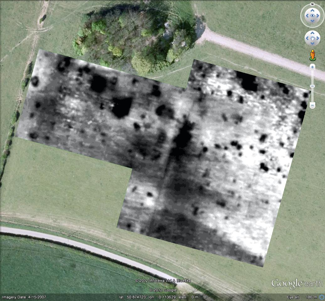
Wouldn't it be really cool if you could walk around your geophysics results, with an image on a screen with your location marked. You could get a good idea of the layout of things on the ground, or easily conduct a guided tour. Well you can! This rather lengthy blog post with describe two methods of doing so, each with their own benefits. This post is a follow on from a previous post, where I describe how to display geophysics results on Google Earth. This post will assume you have already got that far, and you have a geophysics overlay on Google Earth that you wish to walk around.

Google Maps

Unfortunately, the mobile versions of Google Earth and Google Maps do not currently (at the time of writing) support image overlays, so you can't just put a kmz on your phone and view it. What they can do is view vector graphics, but not directly from a file. Say you wanted to display some vector graphics (i.e. lines or placemarks), first save them to a kml file. Now go to Google Maps (on your computer, not your mobile device), where you will see a button called 'My places'. Clicking that will show you a list of vector files you have uploaded to Google. You can upload a new one by 'CRATE MAP' button. Give it a name, and select whether or not you want it publicly available, then click the import link and upload your kml file. Finally press the 'DONE' button.

Now onto your mobile device. Turn the GPS on if necessary, and load up Google Maps. Press the layers button at the top. One of the options will be 'My Maps'. Selecting this should bring up a list of the files you have uploaded. Selecting one will display it on Google Maps. If only this worked with image overlays, that would be nice and easy. You could of course draw some points, lines and polygons over features on your geophysics results and use that, but that would be cheating. We want a real image overlay! So here we go, two methods of doing just that.

Method 1 : With A Laptop


The first method will use a laptop, running Google Earth. I am assuming that the Windows operating system is used. Apologies to those that don't use it. Using a laptop means displaying the image overlays is not a problem, but causes us two other problems.


Firstly, Google Earth needs the internet to display it's own imagery. If you somehow have access to WiFi in the middle of a field, well that's nice for you, but most likely you won't. The easiest way to deal with this is tethering to a mobile device. Android devices have the ability to set themselves up as a WiFi hotspot, transferring the data over the phone network. Beware though, if you get a phone free, or cheap, as part of a package from a carrier, it is more than likely that they will have disabled tethering, because they don't like people actually using devices how they want. If you buy a SIM free phone yourself and get a SIM from a carrier separately, you should be alright. Make sure your contract has a monthly data allowance, or you will end up paying a lot of money.

Secondly, laptops don't have a GPS in them, but we can get around that as well. You can buy stand alone GPS units that can connect to a computer via USB. They are quite cheap. Personally, I have a QStarz BT-818XT, which works fine with what I am describing. You may have noticed that Google Earth has some options for dealing with GPS, but personally I have not much luck with it. I tend to use a program called EarthBridge instead. So here are the steps for using it.

1) Plug your GPS into your laptop and turn it on.
2) Check which COM port that your GPS device appears as. You might need to load a driver for it for this to work, which is dependant on the device used. You can see which devices are linked to which COM port in the Device Manager in Windows.
3) Load Google Earth.
4) Load EarthBridge.
5) Go to the 'Preferences' tab in EarthBridge. Change the 'COM Port' to the one observed in the Windows device manager. It is usual for the other connection settings to be 9600/8/None/1/None, but check with the documentation for your GPS to see what the setting should be if you have problems. Set a suitable folder for 'Save KML files to:'. You will need this for later.
6) Press the 'Connect to GPS Device' Button at the bottom. If all is well, you should see some NMEA output and satellite information in the 'GPS Status' tab.
7) Now we want to configure how things appear on Google Earth, so go to the 'KML Output Settings' tab. UNTICK the checkboxes marked 'Use Altitude Data If Available', 'Show the track information' and 'Fly To Placemark on Update'. Get rid of the placemark title and disable 'Show Speed'. Now you can press the 'Start' button at the bottom.
8) Go to Google Earth and in the 'Add' menu, select 'Network Link'. Browse to the directory you noted in point 5, and select the earthbridge-data.kml file. You should now hopefully see a dot representing your position appear on Google Earth, woohoo! The dot is a bit chunky, it could do with being a cross-hair, but it will do.


On the plus side, you have all the functionality of the full version of Google Earth, with turning layers on and off, and scrolling around however much you wish. On the minus side, carrying around a laptop with a GPS dangling from it is clunky, plus it is never easy to see a laptop screen outdoors.

Method 2 : With a Mobile Device

If we don't like lugging a laptop around a field, you can use a more portable device, such as a smartphone or tablet. Here, I will be assuming that an android device is used, but a method similar to this may work with other mobile operating systems. Unlike with the laptop, we will have no problem with the GPS or internet access, but we will have problems displaying the image in the first place. As mentioned above, the mobile versions of Google Earth/Maps don't currently support image overlays, oh woe and thrice woe. There is a way to do it though, but it is a dark and convoluted path, not for the faint hearted. The rumours of animal sacrifice involved in these dark arts are entirely fictitious. Fortunately, all of the software involved is free.

1) You will need lots of software for this task. First of all download the OSGEO4W installer. Run it, select 'Advanced Install', then 'Install from Internet', then 'All Users' and select the directory into which you want all this software installed, remembering this for later. Use whatever 'Local Package Directory' it chooses, unless there is a problem, then tell it what kind of internet setup you have. You will see various categories of software that you can install.
2) From the Commandline_Utilities category, make sure that gdal and proj are selected. From the Desktop category, make sure that qgis is selected. Everything else needed should be automatically selected as dependencies of those. pressing the Next button will start the install.
3) Even more software, download OruxMapsDesktop. It doesn't have an installer since it is a java application, so just unpack it from its zip file and put the directory somewhere.
4) Yet more software. Install the OruxMaps application on your android mobile device. You can search for it in the android marketplace. It's free.
5) Now we have all the software we need we can begin. Start by creating a directory somewhere where you can put all of the files associated with this. I have used the directory E:\Data\gis\oruxtest, so if you see that directory in the following explanations, you will know what that means, and you can replace that with whatever directory you are using.
6) The area that you are viewing on your mobile device will be limited to a single image that you can save from Google Earth as a jpg, so you need to pick the area you are viewing carefully. This means no scrolling around a large area, and you can't turn layers on and off. Bear in mind that if the area you are viewing is too large, you wont see much resolution on the geophysics, and wont be able to make out the features very well. If the viewing area is too small, you will only have a tiny area to walk around. Don't forget that as well as using your mouse wheel to zoom in and out, you can get a finer control on the zoom by holding down the right mouse button and moving the mouse up and down. Once you have selected the are you wish to walk around, we need to mark it up for georeferencing.
7) You need to add 4 placemarks to the area you are viewing. It helps the next process if they are arranged in a square or rectangle, and it helps you if they are reasonably round numbers. They will also need to be near the corners of the area you are viewing. Right click on your placemarks and select Properties. So they don't get in the way too much, change the icon (button at top right) to a small circle and reduce the scale of the icon ('Style/Colour' tab) to 0.7. Big enough that you can see it on the resulting image, but not too big that it gets in the way. Reduce the scale of the label to 0.1, because we don't need it and don't want it getting in the way. Manually change the Latitude and Longitude so they are roughly in a square or rectangle around the area you are viewing. This is best explained by the example image below, and some real numbers associated with it. If you click on the image below, you will see the four dots, one in each corner. Their coordinates are as follows :

Top-left: 50.914000 Lat 0.022000 Long
Top-right: 50.914000 Lat 0.026000 Long
Bottom-left: 50.911500 Lat 0.022000 Long
Bottom-right: 50.911500 Lat 0.026000 Long

You can see that the numbers have been manually rounded, so as to make a rectangle. You will need to make a note of the numbers that you use for later.

8) Once you have the 4 georeferencing points and the display area perfect, you need to save an image of what you can see, just like in the image above. Go the the 'File' menu, then 'Save', then 'Save Image...', and save the file in the directory that you created in point 5. In this example, the file I have used is called bartest.jpg, so if you see that name later on, you know that you can replace it with your own filename.
9) Now we need to georeference the image. For this, you will need the coordinates that you noted in point 7. If you go to the windows start menu, you should see some of the new software you installed earlier, in the OSGEO4W menu. In that menu, you will find Quantum GIS. Run that now
10) We will need the georeferencer, so go to the 'Plugins' menu, then Georeferencer > Georeferencer.
11) We  need to load the image we have just exported from Google Earth. Click the leftmost icon at the top. If you hover the mouse pointer over it, it should say 'Open raster'. Click on this and select the file you have saved from Google Earth. It should appear on the screen in front of you, with the four small dots near each corner.
12) Click the Zoom In tool up the top. It looks like a magnifying glass with a plus underneath it. Click a couple of times on the dot in the top-left of your image, it should be a lot clearer now. Select the 'Add point' icon at the top. It looks like 3 dots. Aim the mouse pointer at the centre of the circle and click. You will be presented with a window that asks for X and Y coordinates. You will need the coordinates that you noted from point 7. Enter the coordinates relating to this point, with the Latitude going in Y and the Longitude in X. Then hit OK. You need to repeat this for the other three points, which can be reached with the 'Zoom Out' icon, which looks like a magnifying glass with a minus under it, and/or the 'Pan' icon, which looks like a hand. You should end up with something like the image below. Make sure the coordinates are typed in correctly, it is very easy to get them wrong and mess up this part of the process.

13) Once the coordinates for those four points have been entered, click the 'Transformation settings' icon up the top, which looks like a spanner. Set the 'Transformation type' to 'Helmert', the 'Resampling method' to 'Cubic' and the 'Target SRS' to 'EPSG:4326'. The 'Output raster' should be the same filename as the file that you selected to begin with, but with an extension of .tif, so for example 'E:\Data\gis\oruxtest\bartest.jpg' is output as  'E:\Data\gis\oruxtest\bartest.tif'. Once this is all filled in, click OK. An example of how the screen should filled out is given below :

14) Click the 'Start georeferencing' button, which looks like a green play button. This should create a georeferenced image in your directory. This image is a TIF file, which is a standard type of image file, but embedded within this is information as to the geographic location of the image. Embedding this information turns this file into something called a GeoTIF. Find your working folder in windows and open the image. You will probably see that the image has been rotated slightly, with the surrounding area filled in with black. If you find that the image has been rotated a lot, or it has been stretched in one direction, then you have probably entered some of the coordinates wrong, and must start again. If all is well, then we can progress to the next stage. The next stage doesn't seem to like GeoTIFs however, so we must convert it. I wont go into the details of the whys or wherefores too much, I will just tell you what you need to do.
15) To make this easier for the second time around, and to save typing, we are going to create a batch file. In your working directory, create a text file, and put in the following four lines :

c:\osgeo4w\bin\gdal_translate -co "TFW=YES" %1.tif intermediate.tif
c:\osgeo4w\bin\gdal_translate -of PNG %1.tif %1.png
rename intermediate.tfw %1.pgw
del intermediate.tif

If the OSGEO4W software was installed in point 1 was installed anywhere else that c:\osgeo4w, when you will need to change these to the correct location. Save the file, then rename it to 'orux_translate.bat'
16) A new piece of software now, the OSGEO4W shell, in the 'OSGEO4W' menu, there is another menu called 'OSGEO4W' followed by 'OSGeo4W Shell'. Run this.
17) This is like a normal Windows shell, except a few other things are set up for us. We now need to get to our working directory. In my case, that is 'E:\data\gis\oruxtest', which means I should type :

E:
cd \data\gis\oruxtest

18) We can now use the batch file we have created to convert our GeoTIF image into something that the next piece of software can use ("More?", I hear you cry, "You want more?"). Type :

orux_translate bartest

Of course you need to replace bartest with the name of your file, without the extension at the end.
19) Almost there, don't give up now! Now we need to run the OruxMapsDesktop software. In the directory into which you installed the software in point 3, you will find 'OruxMapsDesktop.bat'. Run that.
20) The resulting screen should be filled out as per the image below. Ignore any warnings it brings up along the way. Click 'Calibration file' and select the file in your working directory ending '.pgw'. Click 'Image file' and select the file ending in '.png'. For the DATUM drop down box, select 'WGS 1984: Global Definition'. It is near the bottom of the list.For the PROJECTION drop down box, select 'LATITUDE/LONGITUDE'. In the box next to the 'Destiny Directory' button (the original language for this software is not English, can you tell), enter your working directory. Select 'png format' for the output. Click the 'Create Map' button.

21) If you now look in your working folder, you will see a new directory has appeared which contains an 'xml' and a 'db' file. You need to copy the whole directory, not just the files, to your mobile device. Turn on your mobile device and connect it to your computer with the USB charging cable. A 'Connect to PC' dialog will appear on your mobile device. Select 'Disk Drive'. You should not be able to treat your phone like any other USB mass storage device. Copy the directory you have just created into a directory on your phone called \oruxmaps\mapfiles. Now 'Safely Remove Hardware', just like you would with any normal USB mass storage device.
22) Go out into the field you want to wander about in. Make sure GPS is activated on your mobile device, and then load the OruxMaps App.Select Map offline, press 'Reset Map Sources' if your map is not there, then select your map. You should see something like in the image below. Press the wiggly line up the top and select 'Start GPS', and away you go, you can wander about your geophysics on your phone. Huzzah! The default cursor of the giant arrow is a bit of a blunt instrument for walking around in such a manner. You can select a better cursor in Settings > User Interface > Cursor > Cursor Icon. 'neodraig2' seems to be the best one there currently.

On the plus side you can walk around your geophysics using a genuinely portable device with a screen that works well outside. On the downside, you are limited to a single Google Earth image to walk around, and you can't do anything with layers. Plus, it's a hideously complicated process to do each image. If you thought it was complex to reproduce what I have done, imagine what it was like working out how to do it in the first place!

Accuracy

You might think that this is a good way to position trenches, but you would be wrong. Whilst survey grade GPS systems will get you to within a cm of where you want. consumer grade GPS's will get you within 6-8 metres of where you want, and there doesn't seem to be much available between the two extremes. There is also the Google Earth error. The imagery on Google Earth is not always exactly placed, so you make get another couple of metres error there. So as I mentioned at the start of the post, this is for walking around the geophysics and getting a feel for the place, but you can't rely on it being precise.

Hibernation Time

Well it's getting a bit chilly out there now, too chilly for geophysics, or rather too chilly for me doing geophysics, so this blog will be going quiet over the winter. Hopefully I will have some new and interesting results for you in the spring.